Lecture 7: Troubleshooting Deep Neural Networks

Video

Slides

Notes

Lecture by Josh Tobin. Notes transcribed by James Le and Vishnu Rachakonda.

In traditional software engineering, a bug usually leads to the program crashing. While this is annoying for the user, it is critical for the developer to inspect the errors to understand why. With deep learning, we sometimes encounter errors, but all too often, the program crashes without a clear reason why. While these issues can be debugged manually, deep learning models most often fail because of poor output predictions. What’s worse is that when the model performance is low, there is usually no signal about why or when the models failed.

A common sentiment among practitioners is that they spend 80–90% of time debugging and tuning the models and only 10–20% of time deriving math equations and implementing things. This is confirmed by Andrej Kaparthy, as seen in this tweet.

1 - Why Is Deep Learning Troubleshooting Hard?

Suppose you are trying to reproduce a research paper result for your work, but your results are worse. You might wonder why your model’s performance is significantly worse than the paper that you’re trying to reproduce?

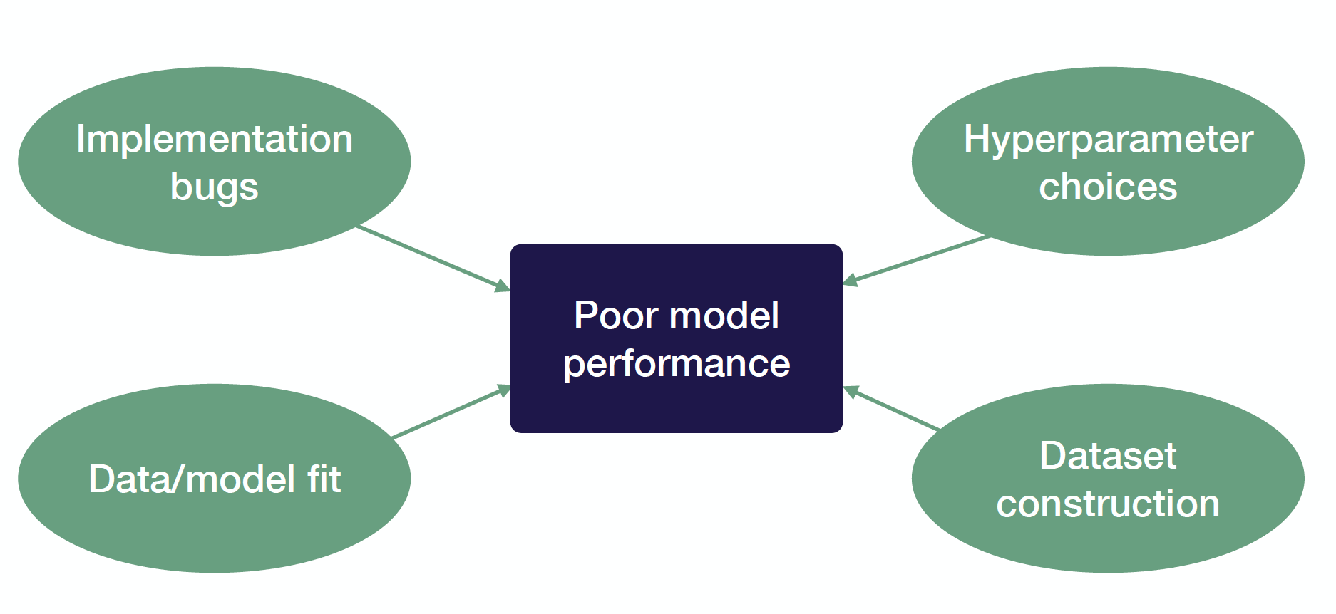
Many different things can cause this:

It can be implementation bugs. Most bugs in deep learning are actually invisible.
Hyper-parameter choices can also cause your performance to degrade. Deep learning models are very sensitive to hyper-parameters. Even very subtle choices of learning rate and weight initialization can make a big difference.
Performance can also be worse just because of data/model fit. For example, you pre-train your model on ImageNet data and fit it on self-driving car images, which are harder to learn.
Finally, poor model performance could be caused not by your model but your dataset construction. Typical issues here include not having enough examples, dealing with noisy labels and imbalanced classes, splitting train and test set with different distributions.

2 - Strategy to Debug Neural Networks

The key idea of deep learning troubleshooting is: Since it is hard to disambiguate errors, it’s best to start simple and gradually ramp up complexity.

This lecture provides a decision tree for debugging deep learning models and improving performance. This guide assumes that you already have an initial test dataset, a single metric to improve, and target performance based on human-level performance, published results, previous baselines, etc.

3 - Start Simple

The first step is the troubleshooting workflow is starting simple.

Choose A Simple Architecture

There are a few things to consider when you want to start simple. The first is how to choose a simple architecture. These are architectures that are easy to implement and are likely to get you part of the way towards solving your problem without introducing as many bugs.

Architecture selection is one of the many intimidating parts of getting into deep learning because there are tons of papers coming out all-the-time and claiming to be state-of-the-art on some problems. They get very complicated fast. In the limit, if you’re trying to get to maximal performance, then architecture selection is challenging. But when starting on a new problem, you can just solve a simple set of rules that will allow you to pick an architecture that enables you to do a decent job on the problem you’re working on.

If your data looks like images, start with a LeNet-like architecture and consider using something like ResNet as your codebase gets more mature.
If your data looks like sequences, start with an LSTM with one hidden layer and/or temporal/classical convolutions. Then, when your problem gets more mature, you can move to an Attention-based model or a WaveNet-like model.
For all other tasks, start with a fully-connected neural network with one hidden layer and use more advanced networks later, depending on the problem.

In reality, many times, the input data contains multiple of those things above. So how to deal with multiple input modalities into a neural network? Here is the 3-step strategy that we recommend:

First, map each of these modalities into a lower-dimensional feature space. In the example above, the images are passed through a ConvNet, and the words are passed through an LSTM.
Then we flatten the outputs of those networks to get a single vector for each of the inputs that will go into the model. Then we concatenate those inputs.
Finally, we pass them through some fully-connected layers to an output.

Use Sensible Defaults

After choosing a simple architecture, the next thing to do is to select sensible hyper-parameter defaults to start with. Here are the defaults that we recommend:

Adam optimizer with a “magic” learning rate value of 3e-4.
ReLU activation for fully-connected and convolutional models and Tanh activation for LSTM models.
He initialization for ReLU activation function and Glorot initialization for Tanh activation function.
No regularization and data normalization.

Normalize Inputs

The next step is to normalize the input data, subtracting the mean and dividing by the variance. Note that for images, it’s fine to scale values to [0, 1] or [-0.5, 0.5] (for example, by dividing by 255).

Simplify The Problem

The final thing you should do is consider simplifying the problem itself. If you have a complicated problem with massive data and tons of classes to deal with, then you should consider:

Working with a small training set around 10,000 examples.
Using a fixed number of objects, classes, input size, etc.
Creating a simpler synthetic training set like in research labs.

This is important because (1) you will have reasonable confidence that your model should be able to solve, and (2) your iteration speed will increase.

The diagram below neatly summarizes how to start simple:

4 - Implement and Debug

To give you a preview, below are the five most common bugs in deep learning models that we recognize:

Incorrect shapes for the network tensors: This bug is a common one and can fail silently. This happens many times because the automatic differentiation systems in the deep learning framework do silent broadcasting. Tensors become different shapes in the network and can cause a lot of problems.
Pre-processing inputs incorrectly: For example, you forget to normalize your inputs or apply too much input pre-processing (over-normalization and excessive data augmentation).
Incorrect input to the model’s loss function: For example, you use softmax outputs to a loss that expects logits.
Forgot to set up train mode for the network correctly: For example, toggling train/evaluation mode or controlling batch norm dependencies.
Numerical instability: For example, you get `inf` or `NaN` as outputs. This bug often stems from using an exponent, a log, or a division operation somewhere in the code.

Here are three pieces of general advice for implementing your model:

Start with a lightweight implementation. You want minimum possible new lines of code for the 1st version of your model. The rule of thumb is less than 200 lines. This doesn’t count tested infrastructure components or TensorFlow/PyTorch code.
Use off-the-shelf components such as Keras if possible, since most of the stuff in Keras works well out-of-the-box. If you have to use TensorFlow, use the built-in functions, don’t do the math yourself. This would help you avoid a lot of numerical instability issues.
Build complicated data pipelines later. These are important for large-scale ML systems, but you should not start with them because data pipelines themselves can be a big source of bugs. Just start with a dataset that you can load into memory.

Get Your Model To Run

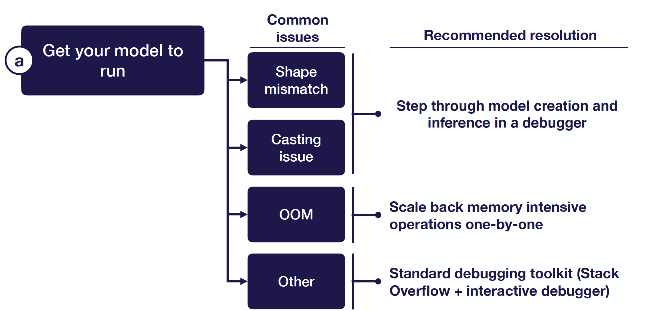
The first step of implementing bug-free deep learning models is getting your model to run at all. There are a few things that can prevent this from happening:

Shape mismatch/casting issue: To address this type of problem, you should step through your model creation and inference step-by-step in a debugger, checking for correct shapes and data types of your tensors.
Out-of-memory issues: This can be very difficult to debug. You can scale back your memory-intensive operations one-by-one. For example, if you create large matrices anywhere in your code, you can reduce the size of their dimensions or cut your batch size in half.
Other issues: You can simply Google it. Stack Overflow would be great most of the time.

Let’s zoom in on the process of stepping through model creation in a debugger and talk about debuggers for deep learning code:

In PyTorch, you can use ipdb — which exports functions to access the interactive IPython debugger.
In TensorFlow, it’s trickier. TensorFlow separates the process of creating the graph and executing operations in the graph. There are three options you can try: (1) step through the graph creation itself and inspect each tensor layer, (2) step into the training loop and evaluate the tensor layers, or (3) use TensorFlow Debugger (tfdb), which does option 1 and 2 automatically.

Overfit A Single Batch

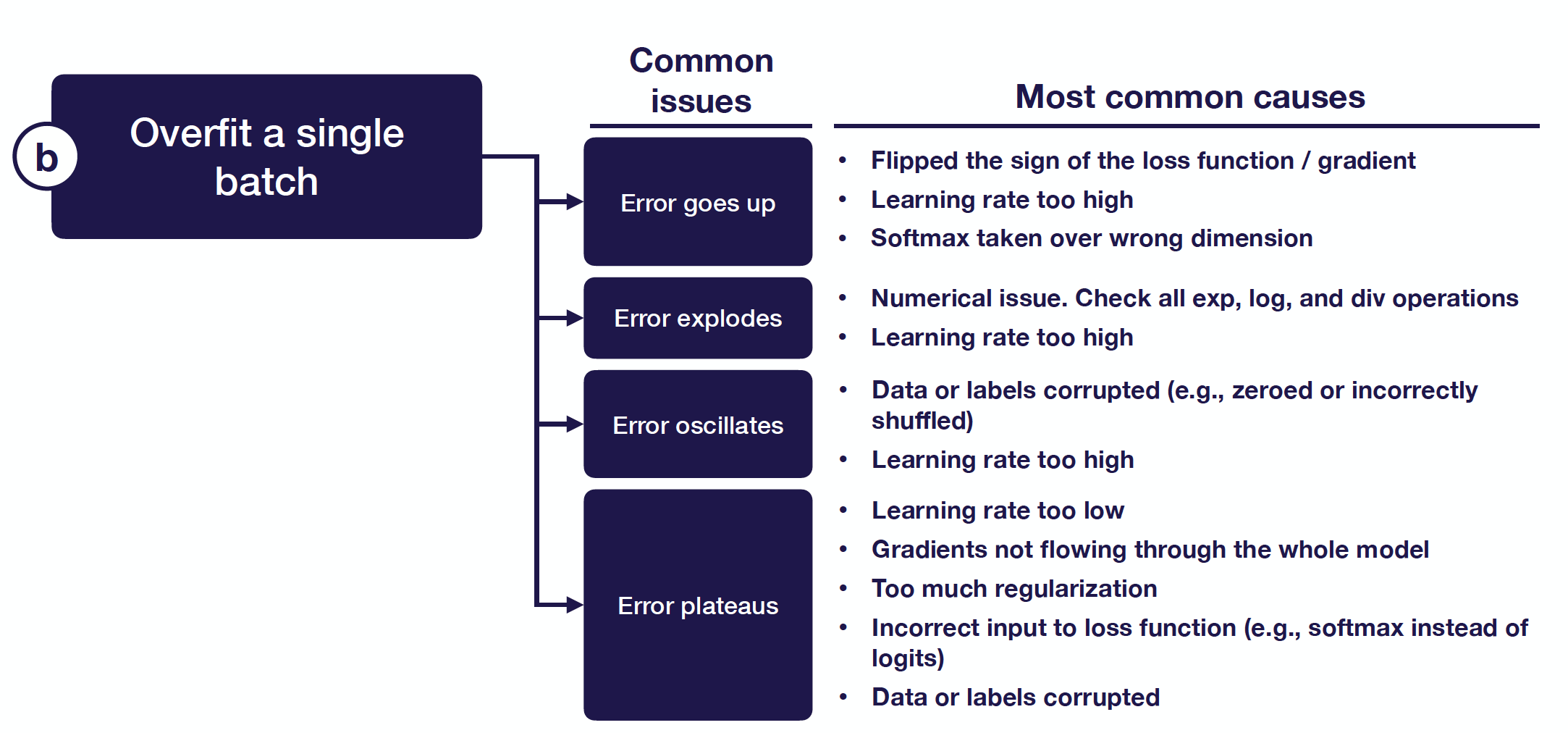
After getting your model to run, the next thing you need to do is to overfit a single batch of data. This is a heuristic that can catch an absurd number of bugs. This really means that you want to drive your training error arbitrarily close to 0.

There are a few things that can happen when you try to overfit a single batch and it fails:

Error goes up: Commonly, this is due to a flip sign somewhere in the loss function/gradient.
Error explodes: This is usually a numerical issue but can also be caused by a high learning rate.
Error oscillates: You can lower the learning rate and inspect the data for shuffled labels or incorrect data augmentation.
Error plateaus: You can increase the learning rate and get rid of regulation. Then you can inspect the loss function and the data pipeline for correctness.

Compare To A Known Result

Once your model overfits in a single batch, there can still be some other issues that cause bugs. The last step here is to compare your results to a known result. So what sort of known results are useful?

The most useful results come from an official model implementation evaluated on a similar dataset to yours. You can step through the code in both models line-by-line and ensure your model has the same output. You want to ensure that your model performance is up to par with expectations.
If you can’t find an official implementation on a similar dataset, you can compare your approach to results from an official model implementation evaluated on a benchmark dataset. You most definitely want to walk through the code line-by-line and ensure you have the same output.
If there is no official implementation of your approach, you can compare it to results from an unofficial model implementation. You can review the code the same as before but with lower confidence (because almost all the unofficial implementations on GitHub have bugs).
Then, you can compare to results from a paper with no code (to ensure that your performance is up to par with expectations), results from your model on a benchmark dataset (to make sure your model performs well in a simpler setting), and results from a similar model on a similar dataset (to help you get a general sense of what kind of performance can be expected).
An under-rated source of results comes from simple baselines (for example, the average of outputs or linear regression), which can help make sure that your model is learning anything at all.

The diagram below neatly summarizes how to implement and debug deep neural networks:

5 - Evaluate

Bias-Variance Decomposition

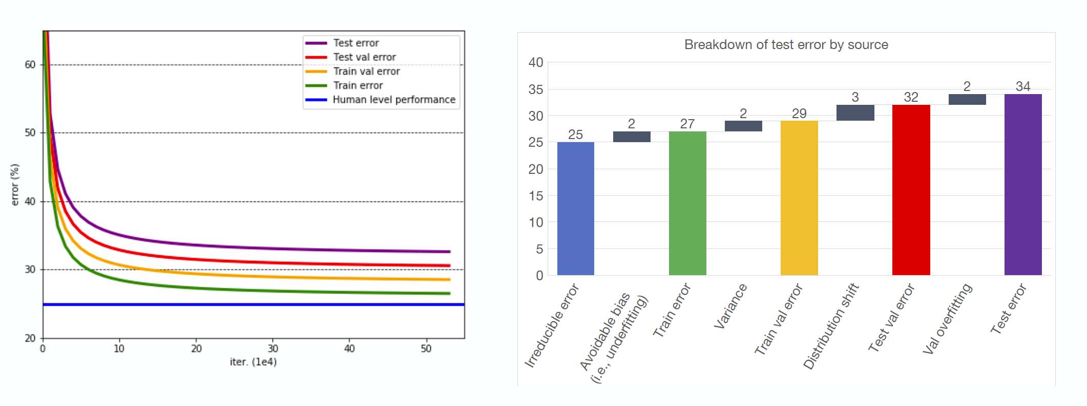
To evaluate models and prioritize the next steps in model development, we will apply the bias-variance decomposition. The bias-variance decomposition is the fundamental model fitting tradeoff. In our application, let’s talk more specifically about the formula for bias-variance tradeoff with respect to the test error; this will help us apply the concept more directly to our model’s performance. There are four terms in the formula for test error:

Test error = irreducible error + bias + variance + validation overfitting

Irreducible error is the baseline error you don’t expect your model to do better. It can be estimated through strong baselines, like human performance.
Avoidable bias, a measure of underfitting, is the difference between our train error and irreducible error.
Variance, a measure of overfitting, is the difference between validation error and training error.
Validation set overfitting is the difference between test error and validation error.

Consider the chart of learning curves and errors below. Using the test error formula for bias and variance, we can calculate each component of test error and make decisions based on the value. For example, our avoidable bias is rather low (only 2 points), while the variance is much higher (5 points). With this knowledge, we should prioritize methods of preventing overfitting, like regularization.

Distribution Shift

Clearly, the application of the bias-variance decomposition to the test error has already helped prioritize our next steps for model development. However, until now, we’ve assumed that the samples (training, validation, testing) all come from the same distribution. What if this isn’t the case? In practical ML situations, this distribution shift often cars. In building self-driving cars, a frequent occurrence might be training with samples from one distribution (e.g., daytime driving video) but testing or inferring on samples from a totally different distribution (e.g., night time driving).

A simple way of handling this wrinkle in our assumption is to create two validation sets: one from the training distribution and one from the test distribution. This can be helpful even with a very small testing set. If we apply this, we can actually estimate our distribution shift, which is the difference between testing validation error and testing error. This is really useful for practical applications of ML! With this new term, let’s update our test error formula of bias and variance:

Test error = irreducible error + bias + variance + distribution shift + validation overfitting

6 - Improve Model and Data

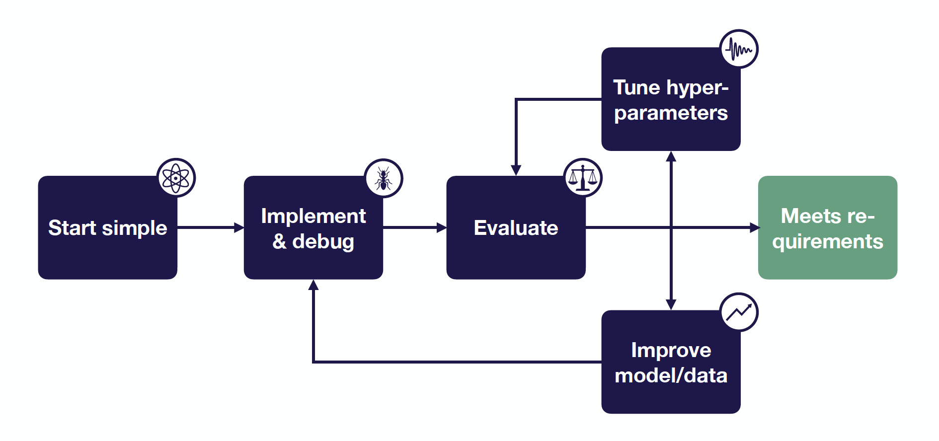
Using the updated formula from the last section, we’ll be able to decide on and prioritize the right next steps for each iteration of a model. In particular, we’ll follow a specific process (shown below).

Step 1: Address Underfitting

We’ll start by addressing underfitting (i.e., reducing bias). The first thing to try in this case is to make your model bigger (e.g., add layers, more units per layer). Next, consider regularization, which can prevent a tight fit to your data. Other options are error analysis, choosing a different model architecture (e.g., something more state of the art), tuning hyperparameters, or adding features. Some notes:

Choosing different architectures, especially a SOTA one, can be very helpful but is also risky. Bugs are easily introduced in the implementation process.
Adding features is uncommon in the deep learning paradigm (vs. traditional machine learning). We usually want the network to learn features of its own accord. If all else fails, it can be beneficial in a practical setting.

Step 2: Address Overfitting

After addressing underfitting, move on to solving overfitting. Similarly, there’s a recommended series of methods to try in order. Starting with collecting training data (if possible) is the soundest way to address overfitting, though it can be challenging in certain applications. Next, tactical improvements like normalization, data augmentation, and regularization can help. Following these steps, traditional defaults like tuning hyperparameters, choosing a different architecture, or error analysis are useful. Finally, if overfitting is rather intractable, there’s a series of less recommended steps, such as early stopping, removing features, and reducing model size. Early stopping is a personal choice; the fast.ai community is a strong proponent.

Step 3: Address Distribution Shift

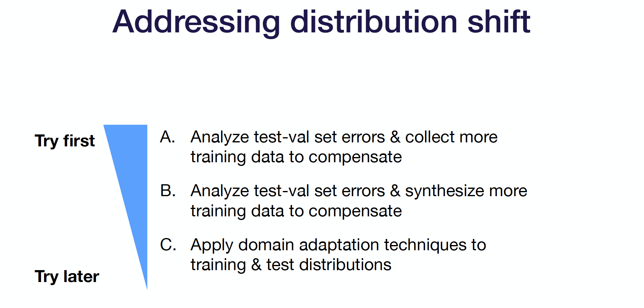
After addressing underfitting and overfitting, If there’s a difference between the error on our training validation set vs. our test validation set, we need to address the error caused by the distribution shift. This is a harder problem to solve, so there’s less in our toolkit to apply.

Start by looking manually at the errors in the test-validation set. Compare the potential logic behind these errors to the performance in the train-validation set, and use the errors to guide further data collection. Essentially, reason about why your model may be suffering from distribution shift error. This is the most principled way to deal with distribution shift, though it’s the most challenging way practically. If collecting more data to address these errors isn’t possible, try synthesizing data. Additionally, you can try domain adaptation.

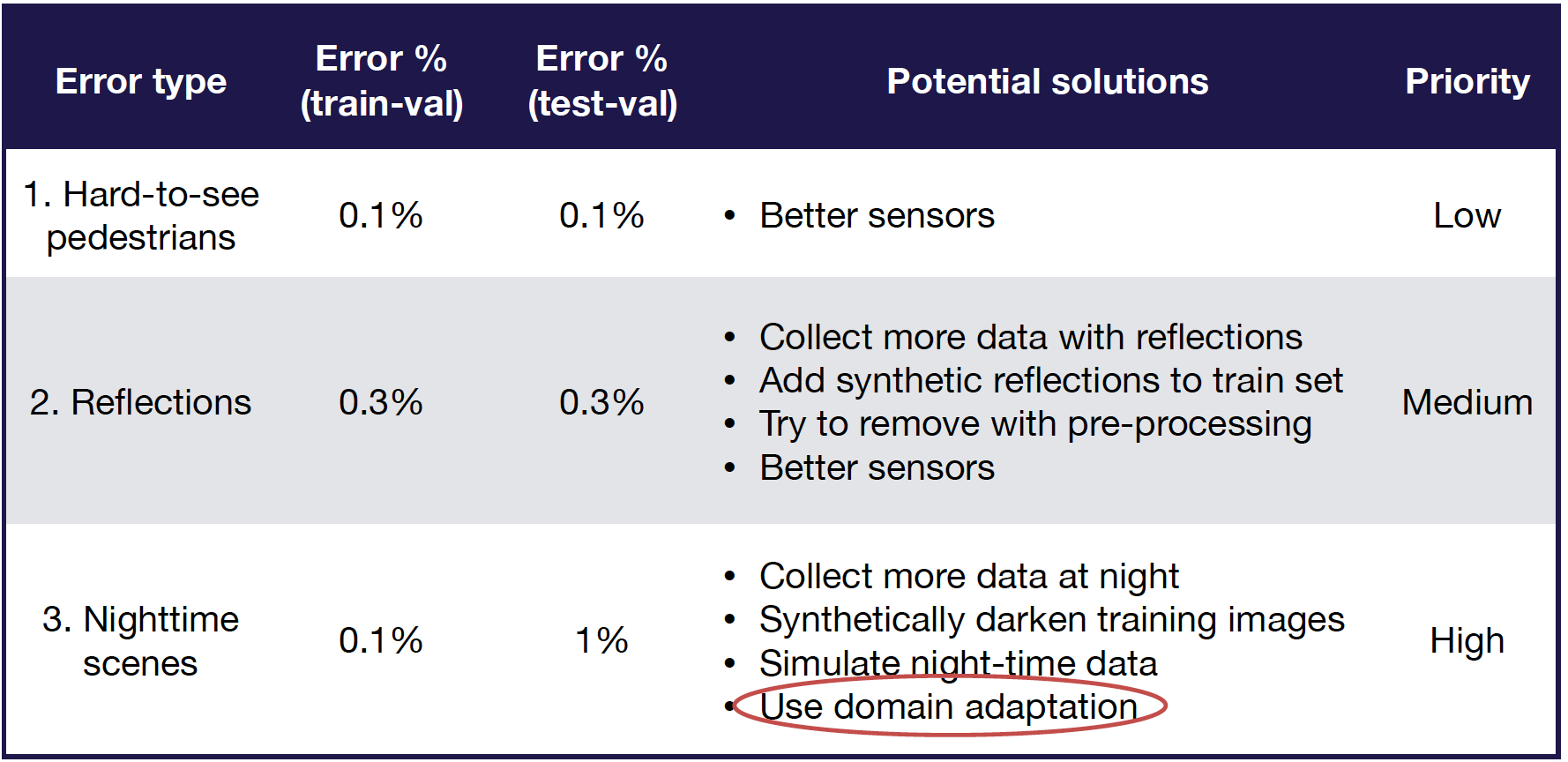
Error Analysis

Manually evaluating errors to understand model performance is generally a high-yield way of figuring out how to improve the model. Systematically performing this error analysis process and decomposing the error from different error types can help prioritize model improvements. For example, in a self-driving car use case with error types like hard-to-see pedestrians, reflections, and nighttime scenes, decomposing the error contribution of each and where it occurs (train-val vs. test-val) can give rise to a clear set of prioritized action items. See the table for an example of how this error analysis can be effectively structured.

Domain Adaptation

Domain adaptation is a class of techniques that train on a “source” distribution and generalize to another “target” using only unlabeled data or limited labeled data. You should use domain adaptation when access to labeled data from the test distribution is limited, but access to relatively similar data is plentiful.

There are a few different types of domain adaptation:

Supervised domain adaptation: In this case, we have limited data from the target domain to adapt to. Some example applications of the concept include fine-tuning a pre-trained model or adding target data to a training set.
Unsupervised domain adaptation: In this case, we have lots of unlabeled data from the target domain. Some techniques you might see are CORAL, domain confusion, and CycleGAN.

Practically speaking, supervised domain adaptation can work really well! Unsupervised domain adaptation has a little bit further to go.

Step 4: Rebalance datasets

If the test-validation set performance starts to look considerably better than the test performance, you may have overfit the validation set. This commonly occurs with small validation sets or lots of hyperparameter training. If this occurs, resample the validation set from the test distribution and get a fresh estimate of the performance.

7 - Tune Hyperparameters

One of the core challenges in hyperparameter optimization is very basic: which hyperparameters should you tune? As we consider this fundamental question, let’s keep the following in mind:

Models are more sensitive to some hyperparameters than others. This means we should focus our efforts on the more impactful hyperparameters.
However, which hyperparameters are most important depends heavily on our choice of model.
Certain rules of thumbs can help guide our initial thinking.
Sensitivity is always relative to default values; if you use good defaults, you might start in a good place!

See the following table for a ranked list of hyperparameters and their impact on the model:

Techniques for Tuning Hyperparameter Optimization

Now that we know which hyperparameters make the most sense to tune (using rules of thumb), let’s consider the various methods of actually tuning them:

Manual Hyperparameter Optimization. Colloquially referred to as Graduate Student Descent, this method works by taking a manual, detailed look at your algorithm, building intuition, and considering which hyperparameters would make the most difference. After figuring out these parameters, you train, evaluate, and guess a better hyperparameter value using your intuition for the algorithm and intelligence. While it may seem archaic, this method combines well with other methods (e.g., setting a range of values for hyperparameters) and has the main benefit of reducing computation time and cost if used skillfully. It can be time-consuming and challenging, but it can be a good starting point.
Grid Search. Imagine each of your parameters plotted against each other on a grid, from which you uniformly sample values to test. For each point, you run a training run and evaluate performance. The advantages are that it’s very simple and can often produce good results. However, it’s quite inefficient, as you must run every combination of hyperparameters. It also often requires prior knowledge about the hyperparameters since we must manually set the range of values.
Random Search: This method is recommended over grid search. Rather than sampling from the grid of values for the hyperparameter evenly, we’ll choose n points sampled randomly across the grid. Empirically, this method produces better results than grid search. However, the results can be somewhat uninterpretable, with unexpected values in certain hyperparameters returned.
Coarse-to-fine Search: Rather than running entirely random runs, we can gradually narrow in on the best hyperparameters through this method. Initially, start by defining a very large range to run a randomized search on. Within the pool of results, you can find N best results and hone in on the hyperparameter values used to generate those samples. As you iteratively perform this method, you can get excellent performance. This doesn’t remove the manual component, as you have to select which range to continuously narrow your search to, but it’s perhaps the most popular method available.
Bayesian Hyperparameter Optimization: This is a reasonably sophisticated method, which you can read more about here and here. At a high level, start with a prior estimate of parameter distributions. Subsequently, maintain a probabilistic model of the relationship between hyperparameter values and model performance. As you maintain this model, you toggle between training with hyperparameter values that maximize the expected improvement (per the model) and use training results to update the initial probabilistic model and its expectations. This is a great, hands-off, efficient method to choose hyperparameters. However, these techniques can be quite challenging to implement from scratch. As libraries and infrastructure mature, the integration of these methods into training will become easier.

In summary, you should probably start with coarse-to-fine random searches and move to Bayesian methods as your codebase matures and you’re more certain of your model.

8 - Conclusion

To wrap up this lecture, deep learning troubleshooting and debugging is really hard. It’s difficult to tell if you have a bug because there are many possible sources for the same degradation in performance. Furthermore, the results can be sensitive to small changes in hyper-parameters and dataset makeup.

To train bug-free deep learning models, we need to treat building them as an iterative process. If you skipped to the end, the following steps can make this process easier and catch errors as early as possible:

Start Simple: Choose the simplest model and data possible.
Implement and Debug: Once the model runs, overfit a single batch and reproduce a known result.
Evaluate: Apply the bias-variance decomposition to decide what to do next.
Tune Hyper-parameters: Use coarse-to-fine random searches to tune the model’s hyper-parameters.
Improve Model and Data: Make your model bigger if your model under-fits and add more data and/or regularization if your model over-fits.

Here are additional resources that you can go to learn more:

Andrew Ng’s “Machine Learning Yearning” book.
This Twitter thread from Andrej Karpathy.
BYU’s “Practical Advice for Building Deep Neural Networks” blog post.

We are excited to share this course with you for free.

We have more upcoming great content. Subscribe to stay up to date as we release it.

We take your privacy and attention very seriously and will never spam you. I am already a subscriber