Lecture 11: Deployment & Monitoring

Video

Deployment:

Monitoring:

Slides

Download slides as PDF

Notes

Download notes as PDF

Lecture by Josh Tobin. Notes transcribed by James Le and Vishnu Rachakonda.

ML in production scales to meet users’ demands by delivering thousands to millions of predictions per second. On the other hand, models in notebooks only work if you run the cells in the right order. To be frank, most data scientists and ML engineers do not know how to build production ML systems. Therefore, the goal of this lecture is to give you different flavors of accomplishing that task.

I - Model Deployment

1 - Types of Deployment

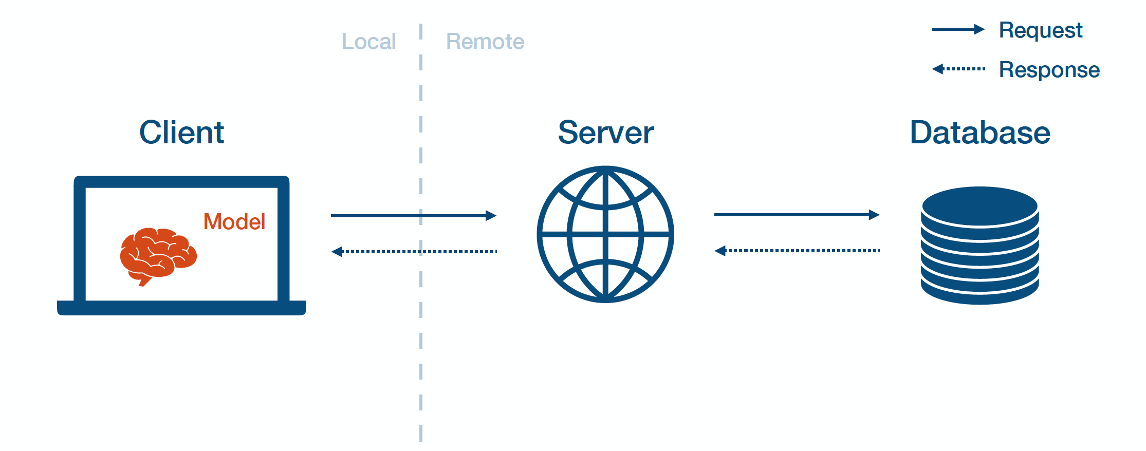
One way to conceptualize different approaches to deploy ML models is to think about where to deploy them in your application’s overall architecture.

• The client-side runs locally on the user machine (web browser, mobile devices, etc..)

• It connects to the server-side that runs your code remotely.

• The server connects with a database to pull data out, render the data, and show the data to the user.

Batch Prediction

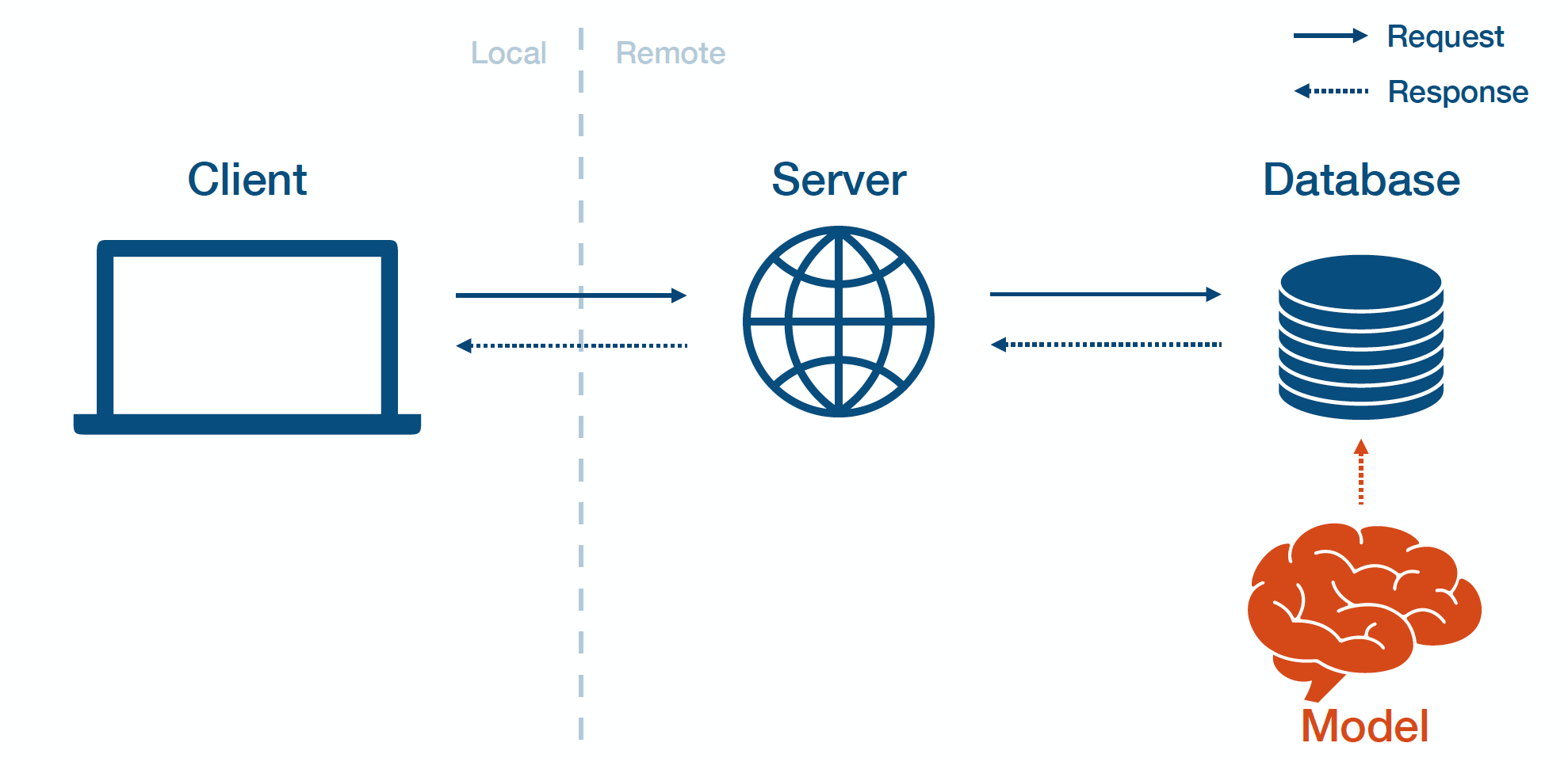
Batch prediction means that you train the models offline, dump the results into a database, then run the rest of the application normally. You periodically run your model on new data coming in and cache the results in a database. Batch prediction is commonly used in production when the universe of inputs is relatively small (e.g., one prediction per user per day).

The pros of batch prediction:

• It is simple to implement.

• It requires relatively low latency to the user.

The cons of batch prediction:

• It does not scale to complex input types.

• Users do not get the most up-to-date predictions.

• Models frequently become “stale” and hard to detect.

Model-In-Service

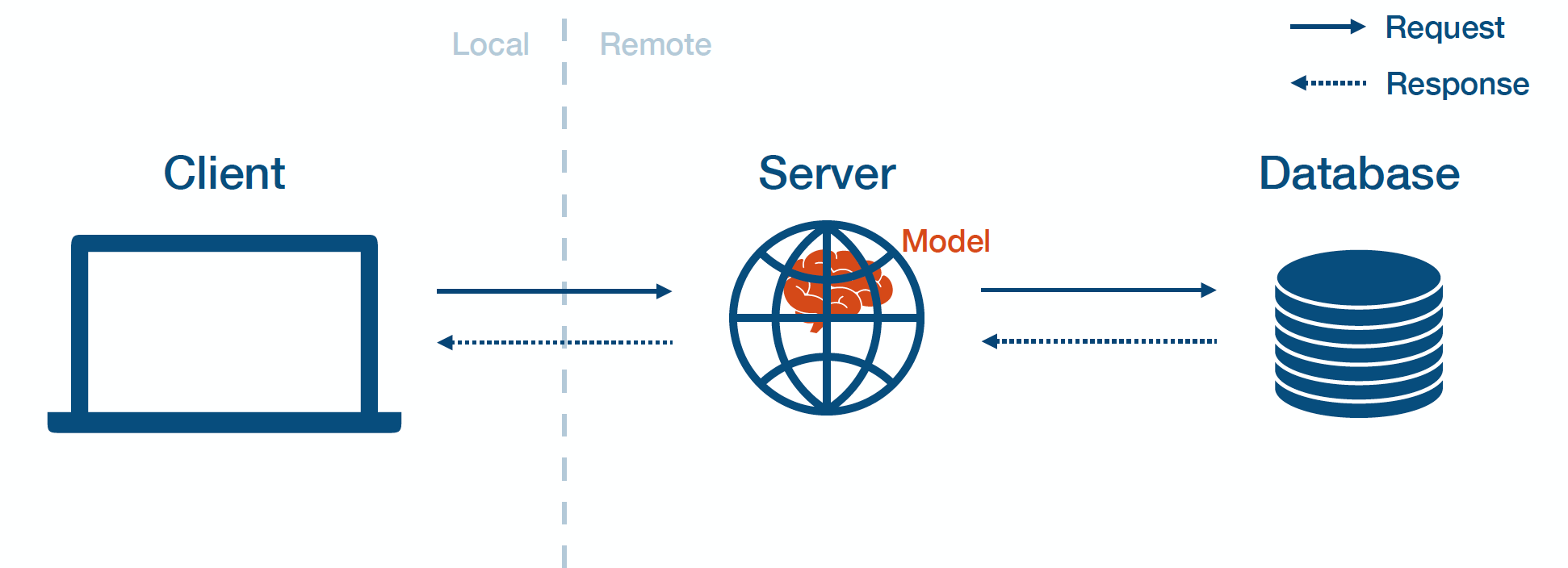
Model-in-service means that you package up your model and include it in the deployed web server. Then, the web server loads the model and calls it to make predictions.

The pros of model-in-service prediction:

• It reuses your existing infrastructure.

The cons of model-in-service prediction:

• The web server may be written in a different language.

• Models may change more frequently than the server code.

• Large models can eat into the resources for your webserver.

• Server hardware is not optimized for your model (e.g., no GPUs).

• Model and server may scale differently.

Model-As-Service

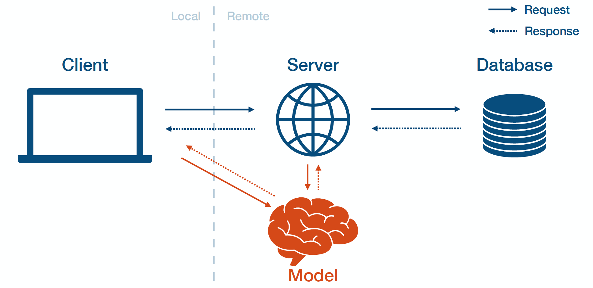
Model-as-service means that you deploy the model separately as its own service. The client and server can interact with the model by making requests to the model service and receiving responses.

The pros of model-as-service prediction:

• It is dependable, as model bugs are less likely to crash the web app.

• It is scalable, as you can choose the optimal hardware for the model and scale it appropriately.

• It is flexible, as you can easily reuse the model across multiple applications.

The cons of model-as-service prediction:

• It adds latency.

• It adds infrastructural complexity.

• Most importantly, you are now on the hook to run a model service...

2 - Building A Model Service

REST APIs

REST APIs represent a way of serving predictions in response to canonically formatted HTTP requests. There are alternatives such as gRPC and GraphQL. For instance, in your command line, you can use curl to post some data to an URL and get back JSON that contains the model predictions.

Sadly, there is no standard way of formatting the data that goes into an ML model.

Dependency Management

Model predictions depend on the code, the model weights, and the code dependencies. All three need to be present on your webserver. For code and model weights, you can simply copy them locally (or write a script to extract them if they are large). But dependencies are trickier because they cause troubles. As they are hard to make consistent and update, your model behavior might change accordingly.

There are two high-level strategies to manage code dependencies:

1. You constrain the dependencies of your model.

2. You use containers.

ONNX

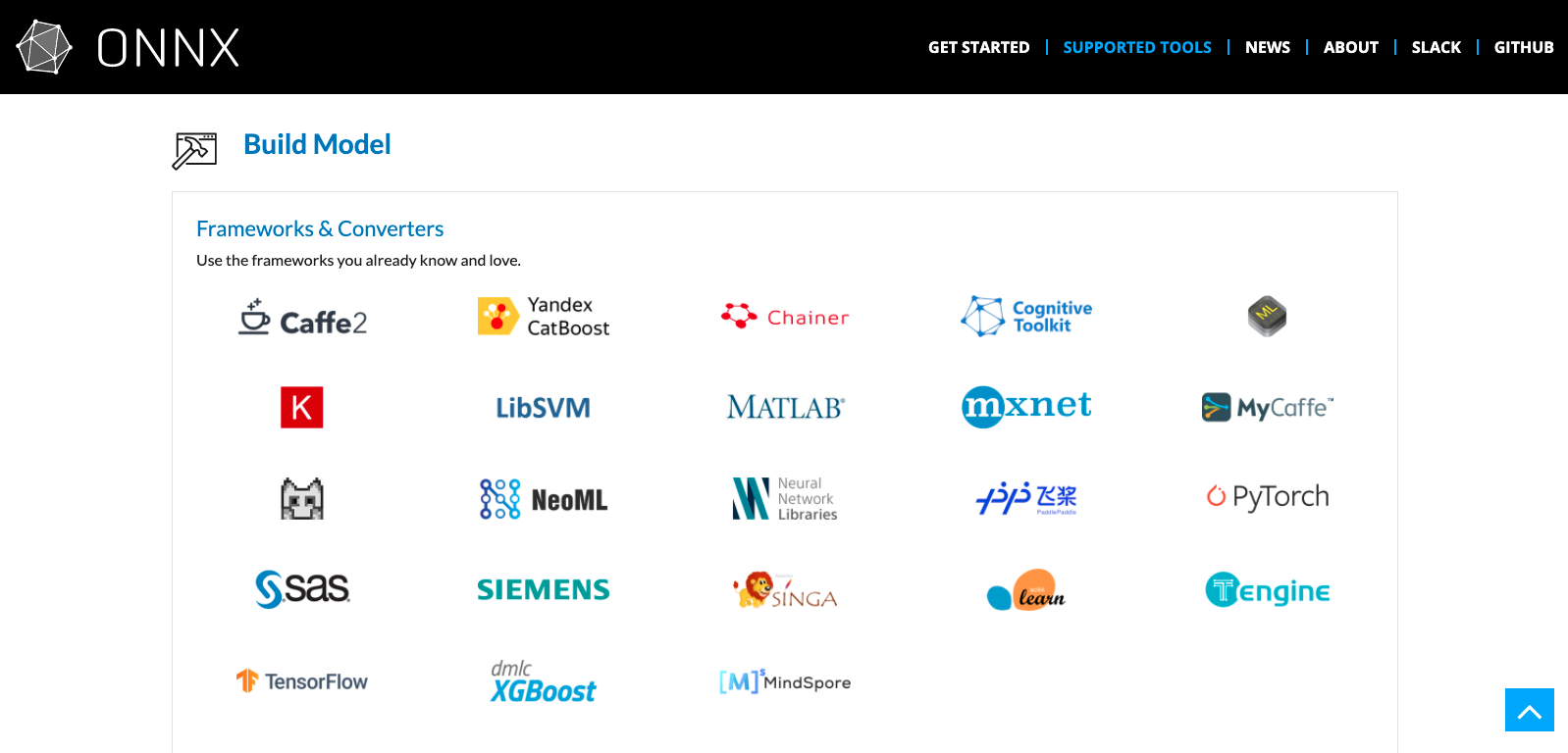
If you go with the first strategy, you need a standard neural network format. The Open Neural Network Exchange (ONNX, for short) is designed to allow framework interoperability. The dream is to mix different frameworks, such that frameworks that are good for development (PyTorch) don’t also have to be good at inference (Caffe2).

• The promise is that you can train a model with one tool stack and then deploy it using another for inference/prediction. ONNX is a robust and open standard for preventing framework lock-in and ensuring that your models will be usable in the long run.

• The reality is that since ML libraries change quickly, there are often bugs in the translation layer. Furthermore, how do you deal with non-library code (like feature transformations)?

Docker

If you go with the second strategy, you want to learn Docker. Docker is a computer program that performs operating-system-level virtualization, also known as containerization. What is a container, you might ask? It is a standardized unit of fully packaged software used for local development, shipping code, and deploying system.

The best way to describe it intuitively is to think of a process surrounded by its filesystem. You run one or a few related processes, and they see a whole filesystem, not shared by anyone.

• This makes containers extremely portable, as they are detached from the underlying hardware and the platform that runs them.

• They are very lightweight, as a minimal amount of data needs to be included.

• They are secure, as the exposed attack surface of a container is extremely small.

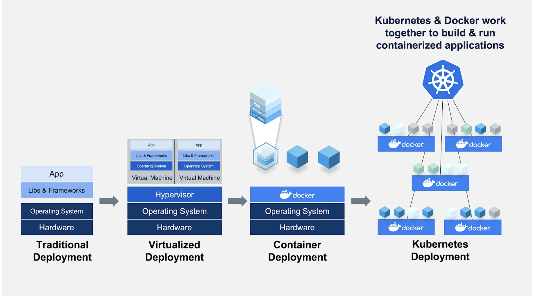
Note here that containers are different from virtual machines.

• Virtual machines require the hypervisor to virtualize a full hardware stack. There are also multiple guest operating systems, making them larger and more extended to boot. This is what AWS / GCP / Azure cloud instances are.

• Containers, on the other hand, require no hypervisor/hardware virtualization. All containers share the same host kernel. There are dedicated isolated user-space environments, making them much smaller in size and faster to boot.

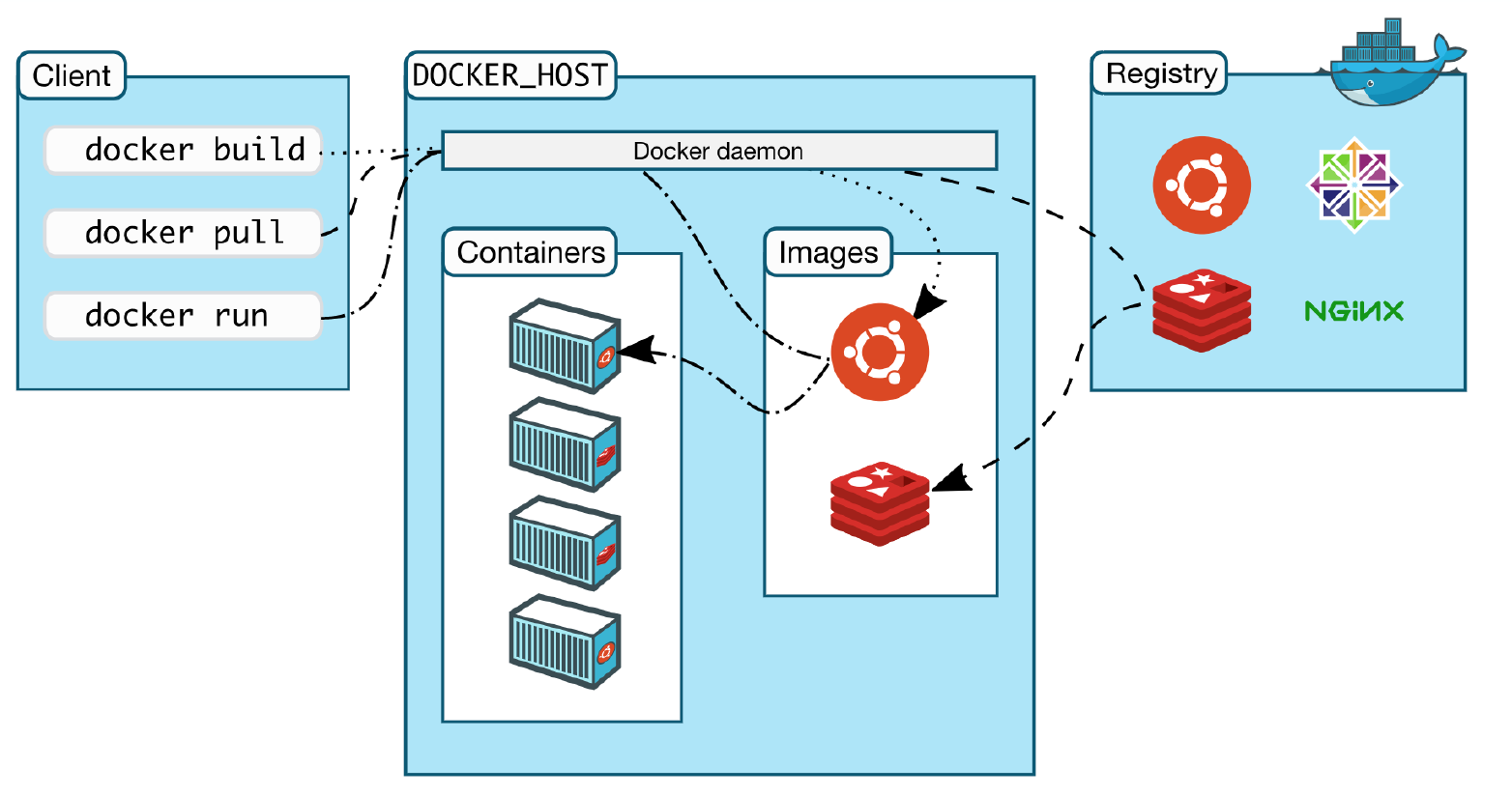
In brief, you should familiarize yourself with these basic concepts:

1. Dockerfile defines how to build an image.

2. Image is a built packaged environment.

3. Container is where images are run inside.

4. Repository hosts different versions of an image.

5. Registry is a set of repositories.

Furthermore, Docker has a robust ecosystem. It has the DockerHub for community-contributed images. It’s incredibly easy to search for images that meet your needs, ready to pull down and use with little-to-no modification.

Though Docker presents how to deal with each of the individual microservices, we also need an orchestrator to handle the whole cluster of services. Such an orchestrator distributes containers onto the underlying virtual machines or bare metal so that these containers talk to each other and coordinate to solve the task at hand. The standard container orchestration tool is Kubernetes.

Performance Optimization

We will talk mostly about how to run your model service faster on a single machine. Here are the key questions that you want to address:

• Do you want inference on a GPU or not?

• How can you run multiple copies of the model at the same time?

• How to make the model smaller?

• How to improve model performance via caching, batching, and GPU sharing?

GPU or no GPU?

Here are the pros of GPU inference:

• You use the same hardware that your model is trained on probably.

• If your model gets bigger and you want to limit model size or tune batch size, you will get high throughput.

Here are the cons of GPU inference:

• GPU is complex to set up.

• GPUs are expensive.

Concurrency

Instead of running a single model copy on your machine, you run multiple model copies on different CPUs or cores. In practice, you need to be careful about thread tuning - making sure that each model copy only uses the minimum number of threads required. Read this blog post from Roblox for the details.

Model distillation

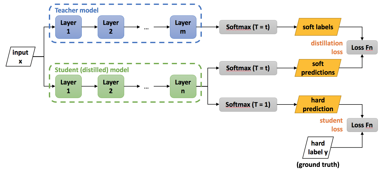
Model distillation is a compression technique in which a small “student” model is trained to reproduce the behavior of a large “teacher” model. The method was first proposed by Bucila et al., 2006 and generalized by Hinton et al., 2015. In distillation, knowledge is transferred from the teacher model to the student by minimizing a loss function. The target is the distribution of class probabilities predicted by the teacher model. That is — the output of a softmax function on the teacher model’s logits.

Distillation can be finicky to do yourself, so it is infrequently used in practice. Read this blog post from Derrick Mwiti for several model distillation techniques for deep learning.

Model quantization

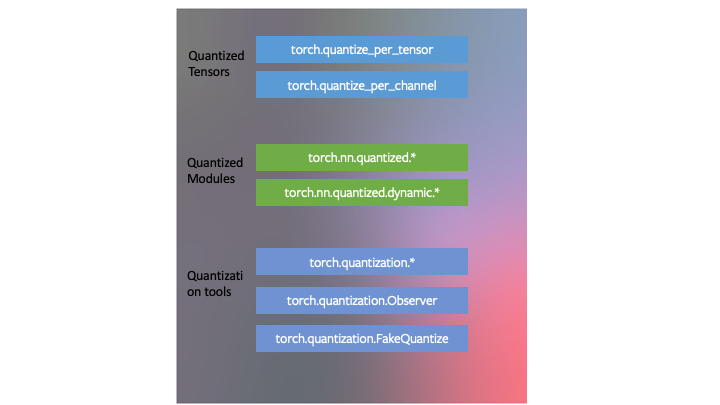
Model quantization is a model compression technique that makes the model physically smaller to save disk space and require less memory during computation to run faster. It decreases the numerical precision of a model’s weights. In other words, each weight is permanently encoded using fewer bits. Note here that there are tradeoffs with accuracy.

• A straightforward method is implemented in the TensorFlow Lite toolkit. It turns a matrix of 32-bit floats into 8-bit integers by applying a simple “center-and-scale” transform to it: W_8 = W_32 / scale + shift (scale and shift are determined individually for each weight matrix). This way, the 8-bit W is used in matrix multiplication, and only the result is then corrected by applying the “center-and-scale” operation in reverse.

• PyTorch also has quantization built-in that includes three techniques: dynamic quantization, post-training static quantization, and quantization-aware training.

Caching

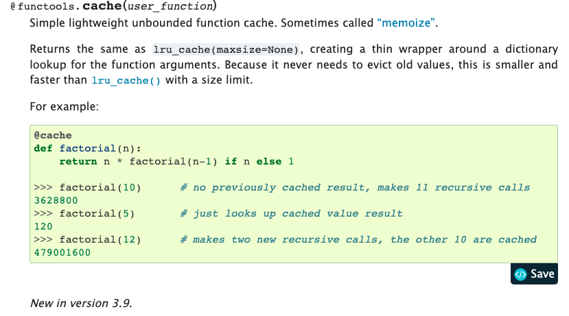
For many ML models, the input distribution is non-uniform (some are more common than others). Caching takes advantage of that. Instead of constantly calling the model on every input no matter what, we first cache the model’s frequently-used inputs. Before calling the model, we check the cache and only call it on the frequently-used inputs.

Caching techniques can get very fancy, but the most basic way to get started is using Python’s functools.

Batching

Typically, ML models achieve higher throughput when making predictions in parallel (especially true for GPU inference). At a high level, here’s how batching works:

• You gather predictions that are coming in until you have a batch for your system. Then, you run the model on that batch and return predictions to those users who request them.

• You need to tune the batch size and address the tradeoff between throughput and latency.

• You need to have a way to shortcut the process if latency becomes too long.

• The last caveat is that you probably do not want to implement batching yourself.

Sharing The GPU

Your model may not take up all of the GPU memory with your inference batch size. Why not run multiple models on the same GPU? You probably want to use a model serving solution that supports this out of the box.

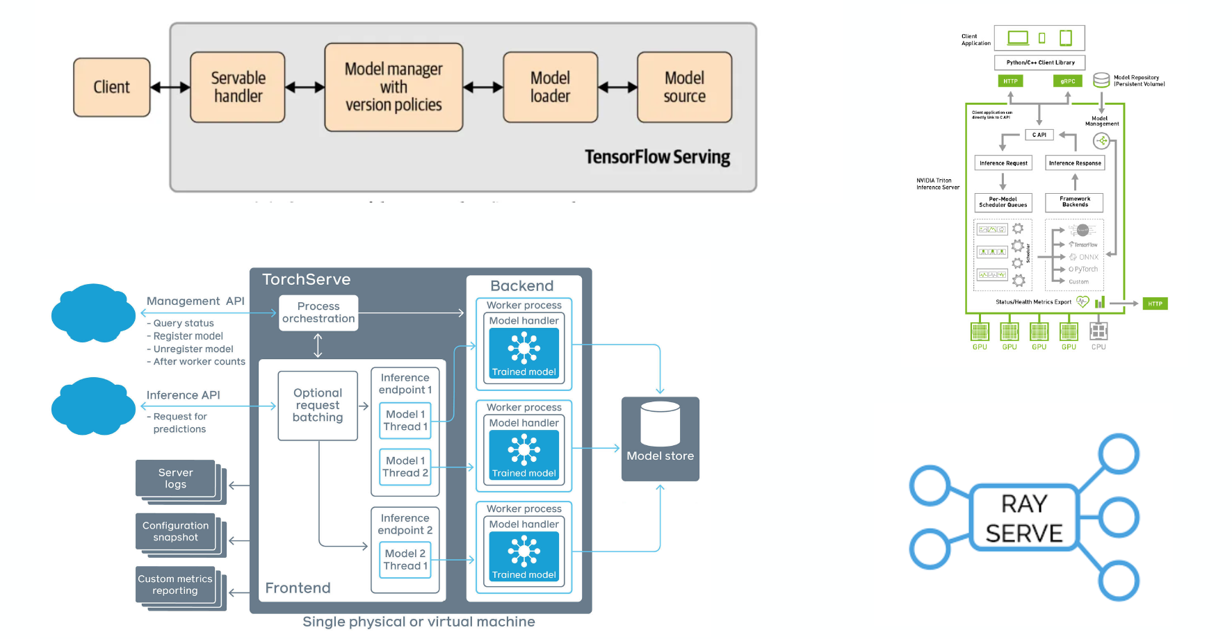
Model Serving Libraries

There are canonical open-source model serving libraries for both PyTorch (TorchServe) and TensorFlow (TensorFlow Serving). Ray Serve is another promising choice. Even NVIDIA has joined the game with Triton Inference Server.

Horizontal Scaling

If you have too much traffic for a single machine, let’s split traffic among multiple machines. At a high level, you duplicate your prediction service, use a load balancer to split traffic, and send the traffic to the appropriate copy of your service. In practice, there are two common methods:

1. Use a container orchestration toolkit like Kubernetes.

2. Use a serverless option like AWS Lambda.

Container Orchestration

In this paradigm, your Docker containers are coordinated by Kubernetes. K8s provides a single service for you to send requests to. Then it divides up traffic that gets sent to that service to virtual copies of your containers (that are running on your infrastructure).

You can build a system like this yourself on top of K8s if you want to. But there are emerging frameworks that can handle all such infrastructure out of the box if you have a K8s cluster running. KFServing is a part of the Kubeflow package, a popular K8s-native ML infrastructure solution. Seldon provides a model serving stack on top of K8s.

Deploying Code As Serverless Functions

The idea here is that the app code and dependencies are packaged into .zip files (or Docker containers) with a single entry point function. All the major cloud providers such as AWS Lambda, Google Cloud Functions, or Azure Functions will manage everything else: instant scaling to 10,000+ requests per second, load balancing, etc.

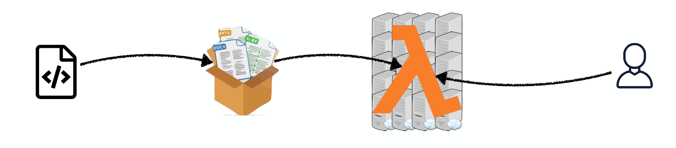
The good thing is that you only pay for compute-time. Furthermore, this approach lowers your DevOps load, as you do not own any servers.

The tradeoff is that you have to work with severe constraints:

1. Your entire deployment package is quite limited.

2. You can only do CPU execution.

3. It can be challenging to build model pipelines.

4. There are limited state management and deployment tooling.

Model Deployment

If serving is how you turn a model into something that can respond to requests, deployment is how you roll out, manage, and update these services. You probably want to be able to roll out gradually, roll back instantly, and deploy pipelines of models. Many challenging infrastructure considerations go into this, but hopefully, your deployment library will take care of this for you.

Managed Options

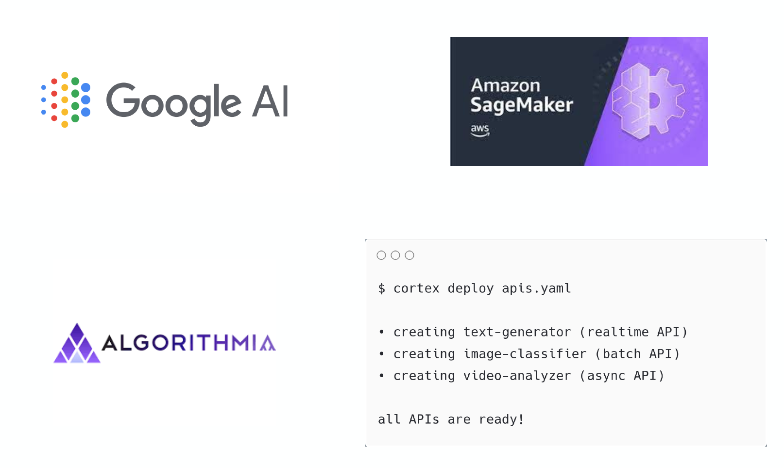
If you do not want to deal with any of the things mentioned thus far, there are managed options in the market. All major cloud providers have ones that enable you to package your model in a predefined way and turn it into an API. Startups like Algorithmia and Cortex are some alternatives. The big drawback is that pricing tends to be high, so you pay a premium fee in exchange for convenience.

Takeaways

• If you are making CPU inference, you can get away with scaling by launching more servers or going serverless.

• Serverless makes sense if you can get away with CPUs, and traffic is spiky or low-volume.

• If you are using GPU inference, serving tools will save you time.

• It’s worth keeping an eye on startups in this space for GPU inference.

3 - Edge Deployment

Edge prediction means that you first send the model weights to the client edge device. Then, the client loads the model and interacts with it directly.

The pros of edge prediction:

• It has low latency.

• It does not require an Internet connection.

• It satisfies data security requirements, as data does not need to leave the user’s device.

The cons of edge prediction:

• The client often has limited hardware resources available.

• Embedded and mobile frameworks are less full-featured than TensorFlow and PyTorch.

• It is challenging to update models.

• It is difficult to monitor and debug when things go wrong.

Tools For Edge Deployment

TensorRT is NVIDIA’s framework meant to help you optimize models for inference on NVIDIA devices in data centers and embedded/automotive environments. TensorRT is also integrated with application-specific SDKs to provide developers a unified path to deploy conversational AI, recommender, video conference, and streaming apps in production.

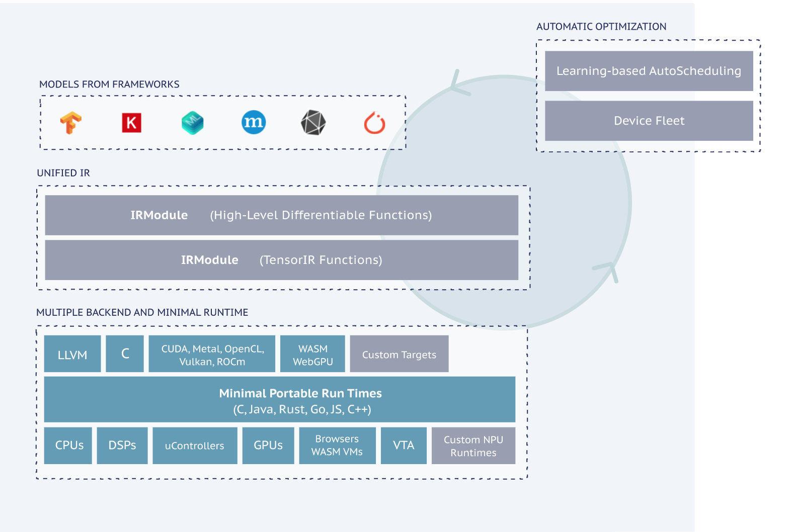
ApacheTVM is an open-source machine learning compiler framework for CPUs, GPUs, and ML accelerators. It aims to enable ML engineers to optimize and run computations efficiently on any hardware backend. In particular, it compiles ML models into minimum deployable modules and provides the infrastructure to automatically optimize models on more backends with better performance.

Tensorflow Lite provides a trained TensorFlow model framework to be compressed and deployed to a mobile or embedded application. TensorFlow’s computationally expensive training process can still be performed in the environment that best suits it (personal server, cloud, overclocked computer). TensorFlow Lite then takes the resulting model (frozen graph, SavedModel, or HDF5 model) as input, packages, deploys, and then interprets it in the client application, handling the resource-conserving optimizations along the way.

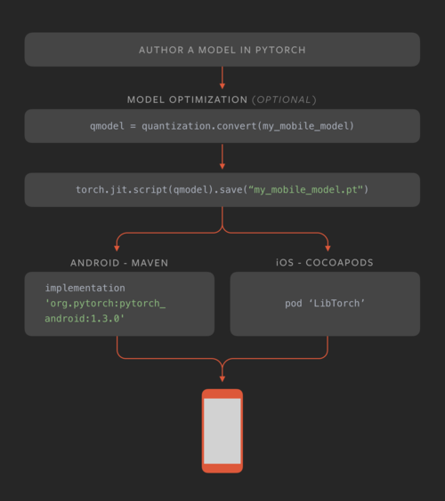
PyTorch Mobile is a framework for helping mobile developers and machine learning engineers embed PyTorch models on-device. Currently, it allows any TorchScript model to run directly inside iOS and Android applications. PyTorch Mobile’s initial release supports many different quantization techniques, which shrink model sizes without significantly affecting performance. PyTorch Mobile also allows developers to directly convert a PyTorch model to a mobile-ready format without needing to work through other tools/frameworks.

JavaScript is a portable way of running code on different devices. Tensorflow.js enables you to run TensorFlow code in JavaScript. You can use off-the-shelf JavaScript models or convert Python TensorFlow models to run in the browser or under Node.js, retrain pre-existing ML models using your data, and build/train models directly in JavaScript using flexible and intuitive APIs.

Core ML was released by Apple back in 2017. It is optimized for on-device performance, which minimizes a model’s memory footprint and power consumption. Running strictly on the device also ensures that user data is kept secure. The app runs even in the absence of a network connection. Generally speaking, it is straightforward to use with just a few lines of code needed to integrate a complete ML model into your device. The downside is that you can only make the model inference, as no model training is possible.

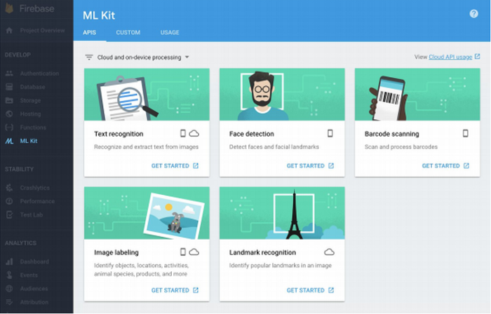
ML Kit was announced by Google Firebase in 2018. It enables developers to utilize ML in mobile apps either with (1) inference in the cloud via API or (2) inference on-device (like Core ML). For the former option, ML Kit offers six base APIs with pertained models such as Image Labeling, Text Recognition, and Barcode Scanning. For the latter option, ML Kit offers lower accuracy but more security to user data, compared to the cloud version.

If you are interested in either of the above options, check out this comparison by the FritzAI team. Additionally, FritzAI is an ML platform for mobile developers that provide pre-trained models, developer tools, and SDKs for iOS, Android, and Unity.

More Efficient Models

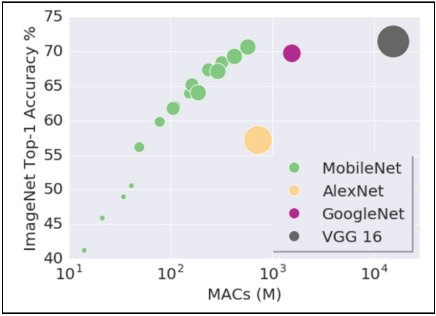
Another thing to consider for edge deployment is to make the models more efficient. One way to do this is to use the same quantization and distillation techniques discussed above. Another way is to pick mobile-friendly model architectures. The first successful example is MobileNet, which performs various downsampling techniques to a traditional ConvNet architecture to maximize accuracy while being mindful of the restricted resources for a mobile or an embedded device. This analysis by Yusuke Uchida explains why MobileNet and its variants are fast.

A well-known case study of applying knowledge distillation in practice is Hugging Face’s DistilBERT, a smaller language model derived from the supervision of the popular BERT language model. DistilBERT removes the toke-type embeddings and the pooler (used for the next sentence classification task) from BERT while keeping the rest of the architecture identical and reducing the number of layers by a factor of two. Overall, DistilBERT has about half the total number of parameters of the BERT base and retains 95% of BERT’s performances on the language understanding benchmark GLUE.

Mindset For Edge Deployment

• It is crucial to choose your architecture with your target hardware in mind. Specifically, you can make up a factor of 2-10 through distillation, quantization, and other tricks (but not more than that).

• Once you have a model that works on your edge device, you can iterate locally as long as you add model size and latency to your metrics and avoid regression.

• You should treat tuning the model for your device as an additional risk in the deployment cycle and test it accordingly. In other words, you should always test your models on production hardware before deploying them for real.

• Since models can be finicky, it’s a good idea to build fallback mechanisms into the application if the model fails or is too slow.

Takeaways

• Web deployment is easier, so only perform edge deployment if you need to.

• You should choose your framework to match the available hardware and corresponding mobile frameworks. Else, you can try Apache TVM to be more flexible.

• You should start considering hardware constraints at the beginning of the project and choose the architectures accordingly.

II - Model Monitoring

Once you deploy models, how do you make sure they are staying healthy and working well? Enter model monitoring.

Many things can go wrong with a model once it’s been trained. This can happen even if your model has been trained properly, with a reasonable validation and test loss, as well as robust performance across various slices and quality predictions. Even after you’ve troubleshot and tested a model, things can still go wrong!

1 - Why Model Degrades Post-Deployment?

Model performance tends to degrade after you’ve deployed a model. Why does this occur? In supervised learning, we seek to fit a function f to approximate a posterior using the data available to us. If any component of this process changes (i.e., the data x), the deployed model can see an unexpectedly degraded performance. See the below chart for examples of how such post-deployment degradations can occur theoretically and in practice:

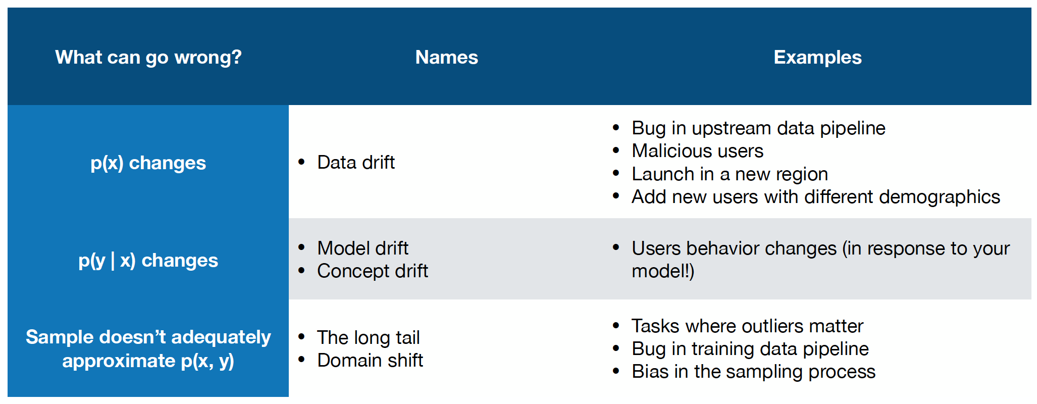
In summary, there are three core ways that the model’s performance can degrade: data drift, concept drift, and domain shift.

1. In data drift, the underlying data expectation that your model is built can unexpectedly change, perhaps through a bug in the upstream data pipeline or even due to malicious users feeding the model bad data.

2. In concept drift, the actual outcome you seek to model, or the relationship between the data and the outcome, may fray. For example, users may start to pick movies in a different manner based on the output of your model, thereby changing the fundamental “concept” the model needs to approximate.

3. Finally, in domain shift, if your dataset does not appropriately sample the production, post-deployment setting, the model’s performance may suffer; this could be considered a “long tail” scenario, where many rare examples that are not present in the development data occur.

2 - Data Drift

There are a few different types of data drift:

• Instantaneous drift: In this situation, the paradigm of the draft dramatically shifts. Examples are deploying the model in a new domain (e.g., self-driving car model in a new city), a bug in the preprocessing pipeline, or even major external shifts like COVID.

• Gradual drift: In this situation, the value of data gradually changes with time. For example, users’ preferences may change over time, or new concepts can get introduced to the domain.

• Periodic drift: Data can have fluctuating value due to underlying patterns like seasonality or time zones.

• Temporary drift: The most difficult to detect, drift can occur through a short-term change in the data that shifts back to normal. This could be via a short-lived malicious attack, or even simply because a user with different demographics or behaviors uses your product in a way that it’s not designed to be used.

While these categories may seem like purely academic categories, the consequences of data shift are very real. This is a real problem that affects many companies and is only now starting to get the attention it merits.

3 - What Should You Monitor?

There are four core types of signals to monitor for machine learning models.

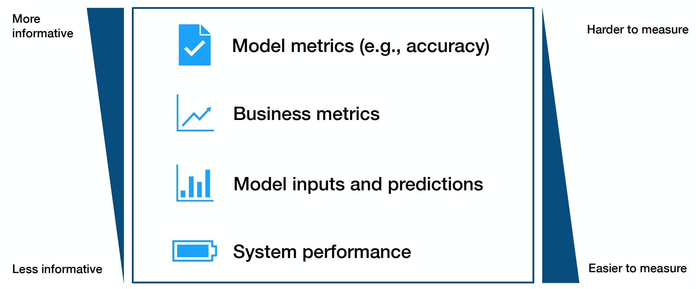
These metrics trade off with another in terms of how informative they are and how easy they are to access. Put simply, the harder a metric may be to monitor, the more useful it likely is.

• The hardest and best metrics to monitor are model performance metrics, though these can be difficult to acquire in real-time (labels are hard to come by).

• Business metrics can be helpful signals of model degradation in monitoring but can easily be confounded by other impactful considerations.

• Model inputs and predictions are a simple way to identify high-level drift and are very easy to gather. Still, they can be difficult to assess in terms of actual performance impact, leaving it more of an art than science.

• Finally, system performance (e.g., GPU usage) can be a coarse method of catching serious bugs.

In considering which metrics to focus on, prioritize ground-truth metrics (model and business metrics), then approximate performance metrics (business and input/outputs), and finally, system health metrics.

4 - How Do You Measure Distribution Changes?

Select A Reference Window

To measure distribution changes in metrics you’re monitoring, start by picking a reference set of production data to compare new data to. There are a few different ways of picking this reference data (e.g., sliding window or fixed window of production data), but the most practical thing to do is to use your training or evaluation data as the reference. Data coming in looking different from what you developed your model using is an important signal to act on.

Select A Measurement Window

After picking a reference window, the next step is to choose a measurement window to compare, measure distance, and evaluate for drift. The challenge is that selecting a measurement window is highly problem-dependent. One solution is to pick one or several window sizes and slide them over the data. To avoid recomputing metrics over and over again, when you slide the window, it’s worth looking into the literature on mergeable (quantile) sketching algorithms.

Compare Windows Using A Distance Metric

What distance metrics should we use to compare the reference window to the measurement window? Some 1-D metric categories are:

1. Rule-based distance metrics (e.g., data quality): Summary statistics, the volume of data points, number of missing values, or more complex tests like overall comparisons are common data quality checks that can be applied. Great Expectations is a valuable library for this. Definitely invest in simple rule-based metrics. They catch a large number of bugs, as publications from Amazon and Google detail.

2. Statistical distance metrics (e.g., KS statistics, KL divergence, D_1 distance, etc.)

   1. KL Divergence: Defined as the expectation of a ratio of logs of two different distributions, this commonly known metric is very sensitive to what happens in the tails of the distribution. It’s not well-suited to data shift testing since it’s easily disturbed, is not interpretable, and struggles with data in different ranges.

   2. KS Statistic: This metric is defined as the max distance between CDFs, which is easy to interpret and is thus used widely in practice. Say yes to the KS statistic!

   3. D1 Distance: Defined as the sum of distances between PDFs, this is a metric used at Google. Despite seeming less principled, it’s easily interpretable and has the added benefit of knowing Google uses it (so why not you?).

An open area of research is understanding the impact of differing drift patterns on distance metrics and model performance. Another open area of research is high-dimensional distance metrics. Some options here are:

1. Maximum mean discrepancy

2. Performing multiple 1D comparisons across the data: While suffering from the multiple hypothesis testing problem, this is a practical approach.

3. Prioritize some features for 1D comparisons: Another option is to avoid testing all the features and only focus on those that merit comparison; for example, those features you know may have shifted in the data.

4. Projections: In this approach, large data points are put through a dimensionality reduction process and then subject to a two-sample statistical test. Reducing the dimensionality with a domain-specific approach (e.g., mean pixel value for images, length of sentence) is recommended.

At a high level, this entire distance metric work aims to identify not just a score for any data shift but also understand its impact on the model. While choosing a metric can be complicated with all the possible options, you should focus on understanding your model’s robustness in a post-deployment scenario.

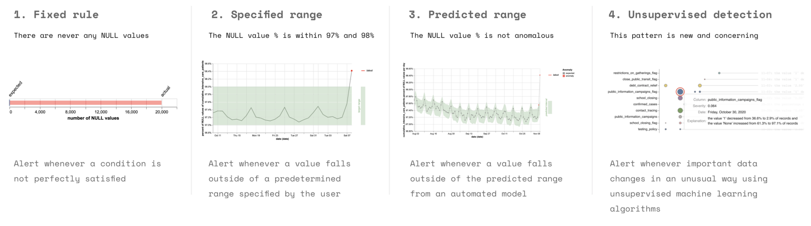
5 - How Do You Tell If A Change Is Bad?

There’s no hard and fast rule for finding if a change in the data is bad. An easy option is to set thresholds on the test values. Don’t use a statistical test like the KS test, as they are too sensitive to small shifts. Other options include setting manual ranges, comparing values over time, or even applying an unsupervised model to detect outliers. In practice, fixed rules and specified ranges of test values are used most in practice.

6 - Tools For Monitoring

There are three categories of tools useful for monitoring:

1. System monitoring tools like AWS CloudWatch, Datadog, New Relic, and honeycomb test traditional performance metrics

2. Data quality tools like Great Expectations, Anomalo, and Monte Carlo test if specific windows of data violate rules or assumptions.

3. ML monitoring tools like Arize, Fiddler, and Arthur can also be useful, as they specifically test models.

7 - Evaluation Store

Monitoring is more central to ML than for traditional software.

• In traditional SWE, most bugs cause loud failures, and the data that is monitored is most valuable to detect and diagnose problems. If the system is working well, the data from these metrics and monitoring systems may not be useful.

• In machine learning, however, monitoring plays a different role. First off, bugs in ML systems often lead to silent degradations in performance. Furthermore, the data that is monitored in ML is literally the code used to train the next iteration of models.

Because monitoring is so essential to ML systems, tightly integrating it into the ML system architecture brings major benefits. In particular, better integrating and monitoring practices, or creating an evaluation store, can close the data flywheel loop, a concept we talked about earlier in the class.

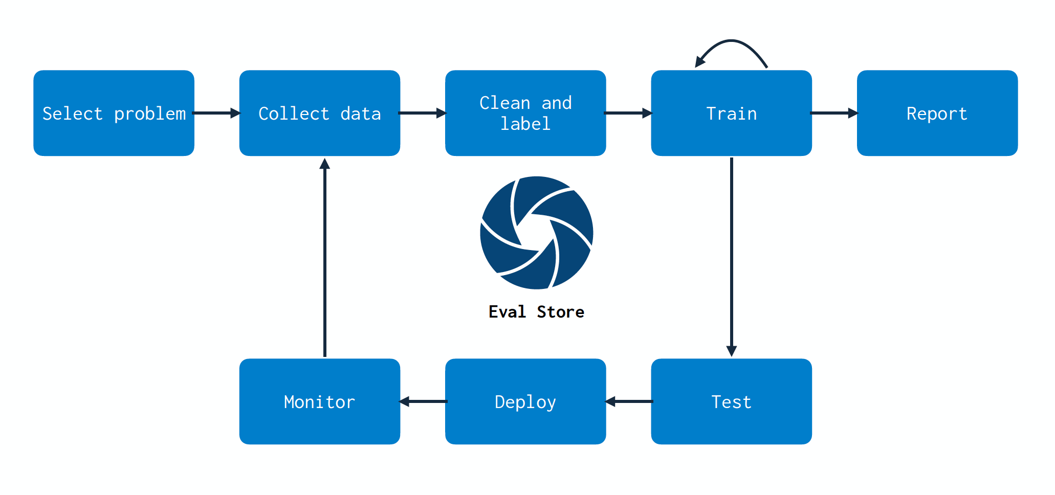
As we build models, we create a mapping between data and model. As the data changes and we retrain models, monitoring these changes doesn’t become an endpoint--it becomes a part of the entire model development process. Monitoring, via an evaluation store, should touch all parts of your stack. One challenge that this process helps solve is effectively choosing which data points to collect, store, and label. Evaluation stores can help identify which data to collect more points for based on uncertain performance. As more data is collected and labeled, efficient retraining can be performed using evaluation store guidance.

Conclusion

In summary, make sure to monitor your models!

• Something will always go wrong, and you should have a system to catch errors.

• Start by looking at data quality metrics and system metrics, as they are easiest.

• In a perfect world, the testing and monitoring should be linked, and they should help you close the data flywheel.

• There will be a lot of tooling and research that will hopefully come soon!

We are excited to share this course with you for free.

We have more upcoming great content. Subscribe to stay up to date as we release it.

Enter

We take your privacy and attention very seriously and will never spam you. I am already a subscriber